Decoding Minds: EEG Analysis for Schizophrenia Detection

Note: For implementation details, code, and information related to preprocessing, please visit the GitHub repository associated with this study.

Abstract

Millions of people worldwide suffer from schizophrenia, which poses difficult diagnostic challenges. This paper explores the objective diagnosis of the illness by combining machine learning (ML) with the study of Electroencephalography (EEG) data. A variety of classic machine learning (ML) models, ranging from traditional approaches like quadratic discriminant analysis (QDA) and logistic regression (LogReg) to more sophisticated strategies like random forest (RF) and light gradient boosting machine (LGBM), were used for classification, utilizing the characteristic EEG patterns of schizophrenia as biomarkers. Through the use of grid search optimization, each model was refined. Through the use of 5-fold cross-validation, performance was evaluated with an emphasis on measures such ROC AUC, accuracy, precision, and recall. The LGBM model showed itself to be a strong classifier, producing the best results across the board, including a ROC AUC of 95.96% and accuracy of 90%. Gradient Boosting (GB) and Extreme Gradient Boosting (XGB) were close contenders, highlighting the potential of ensemble approaches in improving diagnostic precision. These results signify a step forward in the pursuit of an accurate, less subjective diagnostic approach for schizophrenia, with the potential to extend these methodologies to broader neuropsychiatric applications, thereby augmenting patient care and treatment outcomes.

Keywords: Artificial Intelligence, Schizophrenia Detection, EEG Data Analysis, Machine Learning , Algorithm Performance, Mental Health Diagnostics, Ensemble Methods

1. Introduction

Schizophrenia is a chronic and severe mental disorder that affects about 24 million people globally, to put it in perspective, that is 1 out of 300 individuals in every country¹. It is characterized by distortions in thinking, perception, emotions, language, sense of self, and behavior². Early detection and treatment are crucial for improving the outcomes and helping to manage the symptoms effectively . Diagnosis of schizophrenia has traditionally been difficult due to its dependence on subjective clinical assessments³. Building on existing research, this study paper the combined use of Electroencephalography (EEG) and machine learning to enhance schizophrenia diagnosis, aiming to refine and expand upon the work already done in this field.

Electroencephalography (EEG) has emerged as an important technique in psychiatric research, offering insights into the electrical activity of the brain. Specific EEG patterns, such as atypical brainwave frequencies, are frequently seen in schizophrenia. These patterns are crucial biomarkers that can aid in the identification of the condition, providing a more objective foundation for diagnosis than previous approaches⁴.

To evaluate EEG data, the paper applies machine learning classification techniques. These algorithms are good at recognizing complicated patterns within large datasets, such as EEG recordings⁵. The study intends differentiate EEG data from persons with schizophrenia from those without the disorder by studying these patterns. This technique has the potential to change schizophrenia diagnosis, making it more accurate and less reliant on subjective judgment.

This study has far-reaching implications. A more objective and dependable diagnosis approach can lead to earlier and more effective schizophrenia treatment interventions. Furthermore, the approaches proposed here may be applicable to various neuropsychiatric illnesses, highlighting the adaptability of merging EEG data analysis with machine learning in mental health research. With the potential to improve patient care and treatment outcomes, the integration of EEG data with machine learning presents a promising new avenue in the accurate and timely identification of schizophrenia.

2. Literature Review

Numerous approaches to EEG signal analysis in the setting of schizophrenia have been studied. Due to its effectiveness in modeling EEG signals, frequency-domain feature extraction—specifically, the Fast Fourier Transform (FFT) is extensively employed. Another technique to measure the complexity of EEG time series is Fuzzy Entropy (FuzzyEn), which offers a nonlinear indicator for pattern occurrence probabilities⁶.

The merging of machine learning with EEG analysis has received a lot of interest. Traditional machine learning approaches necessitate substantial signal processing knowledge, which can be challenging. To automate feature extraction from EEG signals, Deep Learning (DL) approaches such as Convolutional Neural Networks (CNNs) and Long Short-Term Memory (LSTM) networks have been introduced. These models, including ResNet-18 and SVM for classification, have showed potential in the diagnosis of schizophrenia⁷.

The research by Chaddad et al. (2023) provides valuable insights, specifically focusing on the application of deep learning models for analyzing EEG signals. Although their study encompasses various neurological disorders, the principles and methodologies are relevant for schizophrenia research. For instance, in the domain of epilepsy, which shares some EEG analysis methodologies with schizophrenia research, deep learning models like simple CNNs have achieved accuracies as high as 98% in seizure detection. In the context of Alzheimer’s disease, deep learning processing systems have reached nearly 90% classification accuracy⁷.

Another study that used EEG data to diagnose schizophrenia used a variety of machine learning models and compared the effectiveness of deep learning (DL) approaches to more conventional ML techniques. With an accuracy of 99.25%, the DL models substantially beat the conventional models, especially the CNN-LSTM architecture with ReLU activation and z-score + L2 normalization. This highlights the value of combining recurrent and convolutional networks for the classification of EEG signals in the diagnosis of schizophrenia⁸. On the other hand, when applied to z-score normalized EEG data, classic machine learning models such as SVM, KNN, and Decision Trees performed worse; the bagging classifier performed the best, with an accuracy of roughly 81.22%. Deep learning has the potential to increase the precision and dependability of medical diagnoses based on EEG signals, as demonstrated by the significant difference in accuracy rates between the advanced DL models and the conventional ML models⁸.

Despite advancements in schizophrenia detection using EEG data and machine learning, significant challenges remain. Traditional ML models, often outperformed by deep learning techniques, present an opportunity for improvement ⁹. My paper aims to explore the performance of these traditional models, employing different preprocessing pipelines, and honing their strengths in interpretability and computational efficiency. Although big and diverse datasets continue to be needed, current work’s goal is to maximize the use of available data through improved algorithms and model tuning. The overall objective is to create machine learning models that are both explicable and correct, providing clear insights into their decision-making processes.

3. Methods

3.1. Dataset

The authors of the study preprocessed the EEG dataset (Part 1 | Part 2) used in this study to a certain extent before releasing it to the public. All 81 subjects’ recordings, 22 new controls and 36 new schizophrenia patient are supplemented with extra information from an earlier study. EEG signals were carefully refined for further analysis as part of the pre-processing protocols set by the publishers. Among these were baseline correction, artifact removal using canonical correlation analysis, outlier channel interpolation, high-pass filtering, re-referencing to the averaged ear lobes, and single trial epoch construction. These actions produced a dataset that was ready to be used in the investigation of event-related potentials (ERPs), which are essential for identifying the specific brain activity associated with schizophrenia.

3.2. Preprocessing

To make more analysis easier, the EEG dataset was first imported and processed. In order to create consolidated time points, each EEG signal, which was initially captured at 1.5-second intervals, was aggregated into 24-second blocks. By guaranteeing that each interval represented a mean over a 24-second period, this method was crucial in creating a consistent framework for interpreting the EEG data. Handling the enormous number of time points for the signals for computational efficiency required special attention, and this was step one. The EEG signals were additionally normalized during the preprocessing stage using z-score normalization. The fact that tree-based models are invariant to this standardization led to the selective application of this normalization. The mitigation of signal amplitude changes was a necessary step, nonetheless, for models where normalization affects performance.

3.3. Feature Extraction

Fast Fourier transform (FFT) and Continuous Wavelet transform (CWT) were combined for the feature extraction process. In order to obtain comprehensive time-frequency information, the CWT approach broke down the EEG signals into 16 scales, ranging from 1 to 32 increasing in increments of 2. Analyzing the non-stationary properties of the EEG data required the use of this approach. FFT was used to convert these time-domain signals into their frequency-domain equivalents, which is complementary. In order to comprehend the brain dynamics linked to schizophrenia, it is important to recognize the prominent frequencies present in the EEG data, which were brought to light by this transition. After executing these changes, we took a variety of statistical characteristics out of every signal that was analyzed, creating a feature set that was extensive enough for further machine learning assessment.

3.4. Machine Learning Techniques

A wide range of traditional machine learning models were used in the study; each was improved for EEG signal classification by grid search optimization. Subsections that follow provide specifics on each model used:

3.4.1. Quadratic Discriminant Analysis (QDA)

QDA, a statistical classifier, was employed with parameters like regularization and covariance. It operates on the principle of decision boundaries shaped as quadratic surfaces. Developed based on the Bayesian decision theory, QDA is effective in cases where classes exhibit distinct variance.¹⁰

3.4.2. Logistic Regression

A fundamental classification approach, Logistic Regression, was utilized with hyperparameters like regularization strength and penalty type. It estimates probabilities using a logistic function, pivotal in binary classification tasks.¹¹

3.4.3. Support Vector Machine (SVC)

SVC was chosen for its effectiveness in high-dimensional spaces. Parameters like kernel type and regularization were optimized. It constructs hyperplanes in a multidimensional space to separate different classes.¹²

3.4.4. K-Nearest Neighbors (KNN)

KNN, a simple yet powerful non-parametric technique, classifies data based on the closest training examples in the feature space, with parameters like the number of neighbors and distance metric.¹³

3.4.5. Decision Tree

A Decision Tree classifier was used for its simplicity and interpretability. Parameters like max depth and min samples split were optimized.¹⁴

3.4.6. Bagging Classifier

This ensemble method integrates multiple base classifiers (decision trees in this paper) to improve stability and accuracy. Key parameters like the number of estimators were optimized.¹⁵

3.4.7. Random Forest

Random Forest, an ensemble of decision trees, was included for its ability to reduce overfitting. It was tuned for criteria like the number of trees and max features.¹⁶

3.4.8. Gradient Boosting Classifier

This method builds an additive model in a forward stage-wise fashion, with each tree correcting the errors of the previous one. It was tuned for max depth.¹⁷

3.4.9. AdaBoost Classifier

AdaBoost, a boosting technique, was utilized where it focuses on correcting the misclassifications of previous classifiers. Parameters like the number of estimators and learning rate were optimized.¹⁸

3.4.10. XGBoost

XGBoost, an implementation of gradient boosted decision trees, was used for its predictive power and speed. It was optimized for depth, learning rate, and other hyperparameters.¹⁹

3.4.11. LightGBM

A gradient boosting framework, LightGBM, is known for its efficiency and high speed. It was tuned for parameters like the number of leaves and learning rate. LightGBM is particularly useful for large datasets.²⁰

4. Results and discussion

4.1. Performance Evaluation Measures

5-fold cross-validation was utilized to assess the efficacy of every machine learning model. Because different parts of the dataset were used for training and testing, a mean score was measured along with the standard deviation, which allowed a more thorough evaluation of each model’s efficacy. Recall, accuracy, precision, and the area under the receiver operating characteristic curve (ROC AUC) were the main performance indicators used to assess the models. A summary of every metric is provided below:

4.1.1. Accuracy

Accuracy measures the proportion of true results (both true positives and true negatives) among the total number of cases examined. It provides a general sense of the model’s overall correctness but doesn’t account for the balance of the classes.

4.1.2. Precision

Precision, or positive predictive value, quantifies the number of true positive predictions divided by the total number of positive predictions (both true positives and false positives). It is crucial in scenarios where the cost of a false positive is high.

4.1.3. Recall

Recall, also known as sensitivity or the true positive rate, measures the proportion of actual positives that are correctly identified as such (e.g., the percentage of actual patients with schizophrenia correctly identified by the model). It is particularly important in medical diagnostics where missing a condition can be critical.

4.1.4. ROC AUC

The area under the ROC curve is a performance measurement for the classification models at various threshold settings. ROC is a probability curve, and AUC represents the degree or measure of separability. A higher AUC value means the model is better at distinguishing between patients with schizophrenia and control subjects.

4.2. Results

4.2.1. Performance Metrics of Machine Learning Models

Model	Accuracy (%)	Precision (%)	Recall (%)	ROC AUC (%)
QDA	65.54 ± 0.93	73.48 ± 1.14	66.21 ± 0.93	69.68 ± 0.98
LogReg	70.04 ± 1.30	72.99 ± 0.88	79.08 ± 1.42	75.81 ± 1.09
DT	72.03 ± 1.68	76.46 ± 1.06	76.81 ± 3.17	72.41 ± 0.66
AdaBoost	75.55 ± 0.47	78.11 ± 0.68	82.08 ± 1.44	82.33 ± 0.81
KNN	75.83 ± 0.54	79.19 ± 0.28	80.76 ± 1.07	82.83 ± 0.49
SVM	78.02 ± 0.34	80.61 ± 0.84	83.23 ± 0.80	85.13 ± 0.53
EBT	85.11 ± 0.57	84.12 ± 1.04	92.56 ± 1.01	92.01 ± 0.48
RF	85.12 ± 0.19	84.13 ± 0.63	92.56 ± 1.35	92.78 ± 0.43
GB	87.65 ± 0.94	86.40 ± 0.89	94.14 ± 0.74	94.94 ± 0.41
XGB	87.93 ± 0.85	87.69 ± 0.69	92.82 ± 0.78	94.70 ± 0.53
LGBM	89.62 ± 0.65	89.25 ± 0.78	93.96 ± 1.19	95.96 ± 0.48

Note: Values are presented as mean ± standard deviation.
Acronyms: QDA (Quadratic Discriminant Analysis), LogReg (Logistic Regression), DT (Decision Tree), AdaBoost (Adaptive Boosting), KNN (K-Nearest Neighbors), SVM (Support Vector Machine), EBT (Ensemble Bagging Trees), RF (Random Forest), GB (Gradient Boosting), XGB (Extreme Gradient Boosting), LGBM (Light Gradient Boosting Machine).

4.2.2. Comparative ROC Curves of Machine Learning Models for Schizophrenia Detection

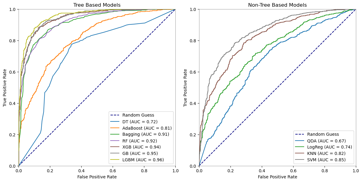figure 1

4.2.3. Precision-Recall Curves of Machine Learning Models for Schizophrenia Detection

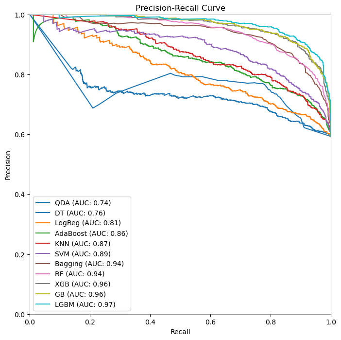figure 2

4.3. Discussion and Conclusion

When it comes to identifying schizophrenia using EEG data, ensemble approaches and advanced algorithms perform better than simpler models, according to the analysis of the performance measures along with the ROC curves. With the best accuracy (89.62%), precision (89.25%), recall (93.96%), and ROC AUC (95.96%), Light Gradient Boosting Machine (LGBM) performs best, indicating a greater capacity to distinguish between the patient and control groups. The ROC curves, which show that LGBM has the highest area under the curve among the models, support this and highlight the model’s predictive power.

Both Extreme Gradient Boosting (XGB) and Gradient Boosting (GB) exhibit strong performance; however, GB performs somewhat better than XGB in terms of recall and ROC AUC, suggesting that it is more adept at detecting true positive situations without raising the false positive rate. This observation is corroborated by the precision-recall curve, which shows that GB and XGB balance recall and precision at different threshold values.

The Random Forest (RF) and Bagging classifiers perform well, almost matching the GB and XGB classifiers in terms of precision and recall. These models, along with LGBM, comprise the top tier of classifiers, implying that ensemble models compared to simpler models like quadratic discriminant analysis, and logistic regression, greatly improve predictive accuracy in EEG-based diagnostic applications.

In conclusion, the study’s findings support the usage of ensemble methods, with LGBM emerging as the most successful model for the task at hand. The consistency of these findings across numerous performance indicators, as well as the ROC curves, show their robustness.

References

1. World Health Organization. (2022, January 10). Schizophrenia. World Health Organization. https://www.who.int/news-room/fact-sheets/detail/schizophrenia ↩

2. American Psychiatric Association. (2020, August). What is Schizophrenia? https://www.psychiatry.org:443/patients-families/schizophrenia/what-is-schizophrenia ↩

3. Jablensky, A. (2010). The diagnostic concept of schizophrenia: Its history, evolution, and future prospects. Dialogues in Clinical Neuroscience, 12(3), 271–287. ↩

4. Newson, J. J., & Thiagarajan, T. C. (2019). EEG Frequency Bands in Psychiatric Disorders: A Review of Resting State Studies. Frontiers in Human Neuroscience, 12, 521. https://doi.org/10.3389/fnhum.2018.00521 ↩

5. Hosseini, M.-P., Hosseini, A., & Ahi, K. (2021). A Review on Machine Learning for EEG Signal Processing in Bioengineering. IEEE Reviews in Biomedical Engineering, 14, 204–218. https://doi.org/10.1109/RBME.2020.2969915 ↩

6. Sun, J., Cao, R., Zhou, M., Hussain, W., Wang, B., Xue, J., & Xiang, J. (2021). A hybrid deep neural network for classification of schizophrenia using EEG Data. Scientific Reports, 11, 4706. https://doi.org/10.1038/s41598-021-83350-6 ↩

7. Chaddad, A., Wu, Y., Kateb, R., & Bouridane, A. (2023). Electroencephalography Signal Processing: A Comprehensive Review and Analysis of Methods and Techniques. Sensors (Basel, Switzerland), 23(14), 6434. https://doi.org/10.3390/s23146434 ↩ ↩²

8. Shoeibi, A., Sadeghi, D., Moridian, P., Ghassemi, N., Heras, J., Alizadehsani, R., Khadem, A., Kong, Y., Nahavandi, S., Zhang, Y.-D., & Gorriz, J. M. (2021). Automatic Diagnosis of Schizophrenia in EEG Signals Using CNN-LSTM Models. Frontiers in Neuroinformatics, 15. https://www.frontiersin.org/articles/10.3389/fninf.2021.777977 ↩ ↩²

9. Rashid, M., Sulaiman, N., P. P. Abdul Majeed, A., Musa, R. M., Ab. Nasir, A. F., Bari, B. S., & Khatun, S. (2020). Current Status, Challenges, and Possible Solutions of EEG-Based Brain-Computer Interface: A Comprehensive Review. Frontiers in Neurorobotics, 14, 25. https://doi.org/10.3389/fnbot.2020.00025 ↩

10. McFarland, H. R., & Richards, D. St. P. (2001). Exact Misclassification Probabilities for Plug-In Normal Quadratic Discriminant Functions. I. The Equal-Means Case. Journal of Multivariate Analysis, 77(1), 21–53. https://doi.org/10.1006/jmva.2000.1924 ↩

11. Cox, D. R. (1958). The Regression Analysis of Binary Sequences. Journal of the Royal Statistical Society. Series B (Methodological), 20(2), 215–242. ↩

12. Cortes, C., & Vapnik, V. (1995). Support-vector networks. Machine Learning, 20(3), 273–297. https://doi.org/10.1007/BF00994018 ↩

13. Cover, T., & Hart, P. (1967). Nearest neighbor pattern classification. IEEE Transactions on Information Theory, 13(1), 21–27. https://doi.org/10.1109/TIT.1967.1053964 ↩

14. Maimon, O. Z., & Rokach, L. (2014). Data Mining With Decision Trees: Theory And Applications (2nd Edition). World Scientific. ↩

15. Breiman, L. (1996). Bagging predictors. Machine Learning, 24(2), 123–140. https://doi.org/10.1007/BF00058655 ↩

16. Breiman, L. (2001). Random Forests. Machine Learning, 45(1), 5–32. https://doi.org/10.1023/A:1010933404324 ↩

17. Friedman, J. H. (2001). Greedy function approximation: A gradient boosting machine. The Annals of Statistics, 29(5), 1189–1232. https://doi.org/10.1214/aos/1013203451 ↩

18. Freund, Y., & Schapire, R. (1999). A Short Introduction to Boosting. https://www.semanticscholar.org/paper/A-Short-Introduction-to-Boosting-Freund-Schapire/c834bddd5e75a64ca9bb80c195cf84345c38bb9b ↩

19. Chen, T., & Guestrin, C. (2016). XGBoost: A Scalable Tree Boosting System. Proceedings of the 22nd ACM SIGKDD International Conference on Knowledge Discovery and Data Mining, 785–794. https://doi.org/10.1145/2939672.2939785 ↩

20. Ke, G., Meng, Q., Finley, T., Wang, T., Chen, W., Ma, W., Ye, Q., & Liu, T.-Y. (2017). LightGBM: A Highly Efficient Gradient Boosting Decision Tree. Advances in Neural Information Processing Systems, 30. https://papers.nips.cc/paper_files/paper/2017/hash/6449f44a102fde848669bdd9eb6b76fa-Abstract.html ↩